On Fuzz Circuits..

The electric guitar was created simply to allow guitarists to compete with the volume of other instruments such as drums etc. In the early days the idea was for electric guitars to sound as close to acoustic guitars as possible. Distortion in amplification then was generally considered to be a ‘problem’.

Aside. What is distortion?

Pure sine waves sound boring or worse unnatural, you just don’t get them in nature. That’s why singers use ‘vibrato’ to make a note ‘interesting’. It’s why we like distortion, it makes a boring plain sound more ‘interesting’.

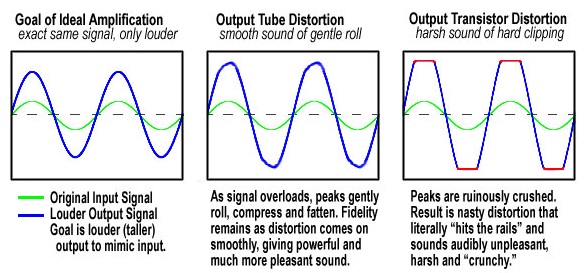
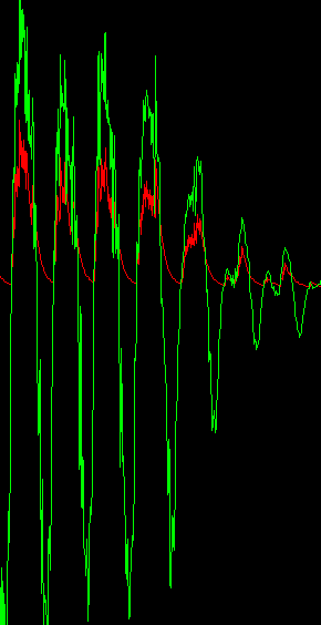
In the above picture the blue ‘sine wave’ represents the perfect signal with no distortion, this represents the output of a ‘perfect’ amplifier. Think of it as being just perfect copy of the signal from the guitar pickups only louder.

However we can see that the red signal is not exactly the same in many places.
A real world amplifier is subject to real world constraints. It can only supply a certain amount of power, and it is not ‘perfect’, nothing is in reality. An amplifier generally has 4 ‘regions’ in which it operates

• The zero crossing or biasing region (green/grey in the diagram above)
  How amplifiers behave around the zero crossing point, exactly where that point is in relation to the input signal and how the amplifier should behave at the bottom end of the input range is dealt with by ‘biasing’.
  I’m not going to discuss it at length (because it’s hard and I don’t understand it properly) except to say that we have ‘stages’ (pre, power etc.) in amplifiers because some components simply won’t work with a small input signal, the signal must be boosted first. People like Eddie Van Halen experimented with this region, and in fact experimentation with (see 6 below) this region is very popular at the moment.
• The linear or ‘good’ region (green)
  This is the region in which the amplifier can be expected to faithfully follow the input signal.
• The Non-linear or saturation region (white)
  This is where the amplifier is at the edge of it’s rated tolerances. A grey area in which the amplifier can sometimes give the right answer, but sometimes does not. This is the area we like, the area in which we get ‘interesting sounds’.
• The unattainable region (red)
  At some point the amplifier simply hasn’t got access to enough ‘juice’ to be able to provide the right signal. We call this ‘the rails’. Some amplifiers can go right up to the rails, and some have a large non-linear region before they hit the rails.

The typical types of distortion we get are numbered in the above diagram:

1. Saturation. This is the type of distortion we’re used to. The valves or transistors in the amplifier are starting to operate in the non-linear region and are behaving unpredictably. You can see here that the general effect is to flatten off (clip) the top of the sine wave by ’rounding it’.
2. Negative signals. The sine wave goes both positive and negative. Sometimes (because of biasing) the valve or transistor will enter the saturation zone at different places (heights, amplitude) in the positive or negative region. This we usually call ‘asymmetric clipping’, and some say it makes things sound more interesting.
3. Here we see that the red line is to the right of the blue line. It’s ‘phase’ is shifted. This is actually very common, but things like guitar chorus pedals and phasers deliberately do this to nice effect. It is one possible feature of amplifier distortion too, but it’s not usually quite so pronounced as it is in say, a chorus pedal. If you want to know exactly why this happens then begin your 4 year journey by asking yourself ‘what is the square root of minus 1?’.
4. Here we see that the signal is not just flattened in the non-linear region, it has ‘interesting’ features. Little ridges or harmonics. In general the more ‘interesting’ things are in the non-linear region the more interesting the sound is. Valve amplifiers tend to be more ‘interesting’ in saturation than transistors are.
5. Transistors are often that ‘good’ that their non-linear zone is tiny. The signal will be linear all the way up to the point where the transistor hits the ‘rails’. This causes perfectly flat clipping. Which sounds sort of artificial to us.
6. Zero crossing distortion is almost always the sign of a bad amplifier design. However it does sometimes sound interesting. And as mentioned a lot of clever effects units are now using this kind of distortion effect.

Some history

In the 50’s rock and roll was in full swing and people were searching for an edgier sound. At some point in the mid 50’s fuzzy guitar tones that had previously been considered wrong, now started to sound good. People would get the sound by deliberately driving their small amplifiers as hard as they could. But the distortion they achieved was unpredictable because it came from a number of sources, the valves or the speakers themselves etc. Amplifiers were deliberately designed NOT to distort, of course that would change by the late 1960’s.

At some point people began modifying valve amplifiers in the most dangerous, ham-fisted, unpredictable and irreversible manner. What was needed was a way of getting that sound easily, safely and and repeatedly. In the early 60’s before things like the Marshall Plexi, this was done using something now very common, a fuzz pedal.

There are several competing narratives about how the first ‘fuzz’ pedal came about but we know that it happened at some time in 1960 or 1961. Let’s just take the first fuzz pedal to be the ‘The Maestro FZ-1 Fuzz-Tone’.

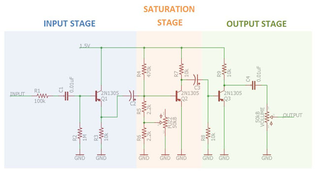
The idea was to replicate what happened in a small amplifier when it was driven too hard.
In that case the valves would ‘saturate’ (see 1 in the wave diagram above) and begin to break up the signal, clipping and distorting it. This circuit tries to emulate that by driving one of the transistors into saturation.

Small Digression

Though transistors and valves are physically different things they work in ‘conceptually’ the same way. Think of a traffic light system. Using a small signal (a light) huge amounts of traffic can be coaxed into flowing, or stopped in its tracks. In valves and transistors the small amount of electricity produced by the guitar pickups is used to ‘coax’ a large amount of electricity to flow, thus ‘amplifying’ the original signal. Under normal operating conditions the output is directly proportional to the input. But in saturation it all starts to go horribly wrong.

The fundamental difference between valves and transistors is how much ‘juice’ they require to operate.
Valves work by causing electrons to literally jump across a gap between several pieces of metal inside a vacuum. Making electrons jump a gap (even in a vacuum) requires a lot of coaxing (high voltage), and once the electrons begin to jump A LOT OF THEM jump (high current).

But since the electrons never leave the conductor (don’t need to jump a gap) in a transistor the amount of voltage and current required for operation is orders of magnitude smaller. Conceptually this doesn’t matter, a valve and a transistor do the exact same job. But how they behave in saturation is very different and has a noticeably different sound. Transistors in saturation sound sharp, fuzzy and artificial. Valves generally sound smoother and richer, essentially because they are ‘less precise’ than solid state components like transistors.

A good analogy is car engines. Both a car with a 10L V12 supercharged engine and one with a 600cc triple cylinder engine may achieve 60mph, but one of them requires far less fuel to do so than the other.
Conversely, one can do 60mph even when going up hill pulling a house behind it, the other one just cannot.
To the onlooker both cars appear the same, they’re both doing 60mph, but how they’ll behave at the edge of their tolerances will vary massively!

Back to the story..

You know what it’s like when someone comes up with some new musical technology, take the Digitech Whammy. Once Tom Morello had used it so well in ‘Killing In The Name’ it was over, nobody else could effectively use it. It had been ‘done’.

For Fuzz this really happened in 1965 when The Rolling Stones released ‘Satisfaction’, featuring a fuzz guitar. The artificial sound of a transistor in saturation had been ‘used up’.

Of course by the late 60’s the much more nuanced (you can’t ‘use it up’ because it sounds kind of different every time) sound of distorted Marshall amplifier had begun to be used by all sorts of bands. But a Plexi was out of reach for most people. Perhaps someone could invent a better fuzz, that sounded more like a Plexi? So what is that sound again?

At some point in 1968 or 1969 the idea of using diode clipping came about.
A diode is a little like a switch, it can be used to cut off flows of electricity (more below).
What if instead of leaving things up to the individual specifications of transistors, we could control the exact place where clipping happens. Essentially we’ll keep the transistor in it’s linear region but somehow artificially set the rails. Perhaps then we’d have more predictable control over what happens in the clipping region because the transistor is still behaving predictably. Better yet we can use a broader range of transistors, including very cheap ones.

I suggest that the first fuzz featuring diode clipping was made by EHX, either the Axis Face, the Foxey Lady or the big muff pi (triangle).
Probably invented by someone called ‘Bill Berko’ or maybe Mike Matthews or possibly Roger Mayer.

What does the Big Muff Pi do?

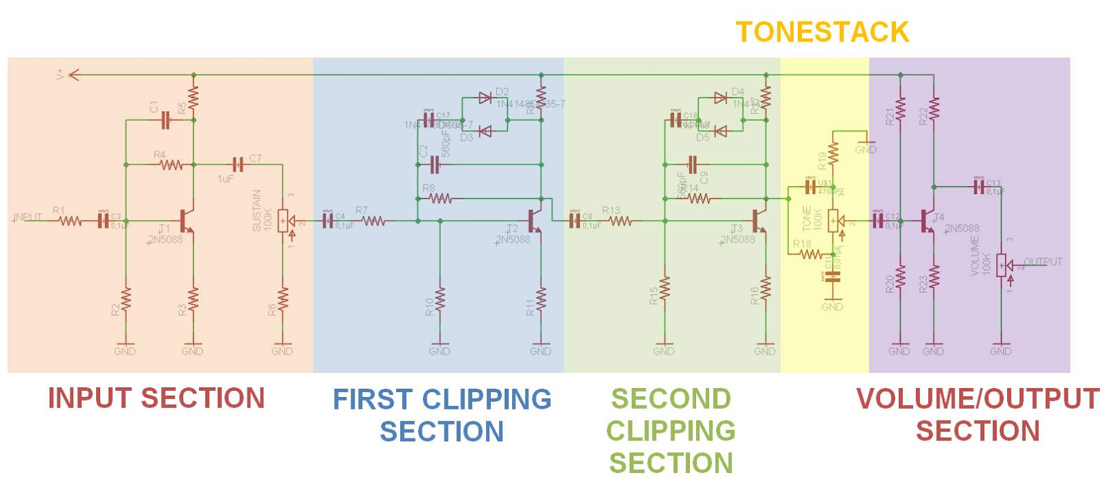
We’ll eventually get to precisely how this works later but for now I’ll just give you the high level.
In the ‘first clipping section’ the transistor is kept in its linear region. It amplifies the original signal such that it is high enough (voltage) for the working range of the diode (for more on this look up ‘ideal diode’ and see below). The resistors and capacitors determine how and where (in relation to the input signal) the diode conducts and does not conduct. The task is to determine exactly where ‘clipping’ occurs using the capacitors and resistors rather than the relying on the biasing and specifications of the transistor.

The Tube Screamer

Before we move on we’ll just take a quick jump forward by 10 years.
Below is the clipping stage of the tube screamer created by Maxon’s Susumu Tamura in 1979.

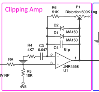
We can see here that it looks very much the same as the clipping section of the Big Muff Pi. There are some resistors, capacitors and two opposed diodes in the feedback loop of an amplifier. In this case the amplifier is not a transistor but an ‘operational amplifier’, a component that by ’79 had become cheap enough to use in place of a transistor. There are many reasons for making this change but let’s just say that op-amps are better amplifiers (a larger useable and stable linear region) than single transistors are.
I show you this because the explanation of how these clipping stages works will use op-amps and not transistors, though there is essentially no difference. all it does is allow us to ignore some components.

Breaking it down

Let’s recap! We want to design a circuit that chops the peaks off waves in a nice way that emulates the way that valves do this when they saturate.

The Big Muff (and pretty much all that has followed) is insanely clever in that it achieves something like this with so few components. What happens if we try to separate out the various functions of these components so that we can easily examine the function of them all and explain how the Big Muff does what it does.

Ideal Diodes

We know that the diodes somehow do the chopping of the waves but let’s start with how to get past the problem of diode ‘forward voltage drop’. Diodes don’t just simply let signals through in one direction and not the other. They only effectively do that when the signal is ABOVE a particular voltage, and they steal a bit of the output voltage too. For germanium diodes this is around 0.3V, just about the max output of a typical guitar pickup. For silicon diodes like the ubiquitous 1N4148 it’s 0.7V, which is far beyond the output of most guitar pickups. In the diagram below we can see we only get an output from the diode when the input signal goes above a particular voltage (around 0.7V in this case), and also that the output signal is not the same size as the input signal. Some voltage is ‘dropped’ (yes, about 0.7V).

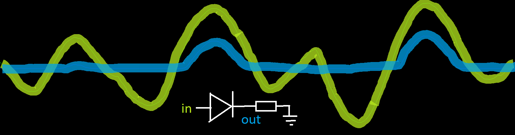
This leaves us with having to amplify (apply gain to) the signal before we can use diodes on it. One way to get past this is to put the diode in the feedback loop of an amplifier like this:

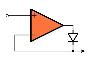
Here the diode is in the feedback loop. The op-amp tries to ensure that the output matches the input. It senses that it has 0.3V on the input but nothing is on the output because the diode will not effectively pass 0.3V. So the op-amp ramps up the output (almost instantly) at 0.7V the silicon diode conducts but the opamp still sees about 0V on the feedback. At about 0.8V the op-amp senses 0.1V at the feedback because the diode has eaten 0.7V, so it continues to ramp up the voltage. At 1V the op-amp now registers 0.3V at the feedback so it stops ramping up the voltage. The feedback is equal to the input. The op-amp has effectively absorbed the forward voltage of the diode. An ideal diode will faithfully pass all positive voltages. Note that if we reverse the polarity of the diode it would pass all negative voltages.

Peak Detection

What we need to do is decide where to chop the tops off the waves. To do this it would be useful to know the maximum voltage the waves reach, in other words we need to detect the ‘peaks’ of the wave. We can do this by using a capacitor and one of our ideal diodes.

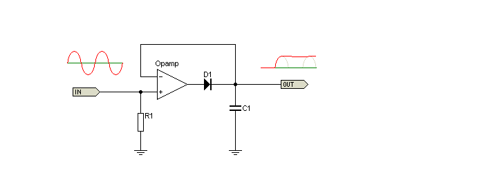
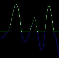
The capacitor charges as the signal gets larger until the peak of the signal is reached. At this point the op-amp detects that the capacitor is at a higher voltage than the input signal and immediately lowers it’s output, but the diode prevents that from happening and the capacitor is left holding it’s last highest charge. The capacitor then leaks slowly until the op-amp starts to raise the output again. This circuit is also sometimes called an ‘envelope follower’ or envelope detector. More specifically an ‘envelope follower’ is a peak detector which can detect both the positive and negative peaks (the whole envelope of the signal).

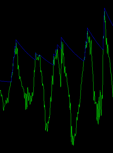
So now we have a measure of roughly where the peaks of our waveform are at any given time (the blue line).
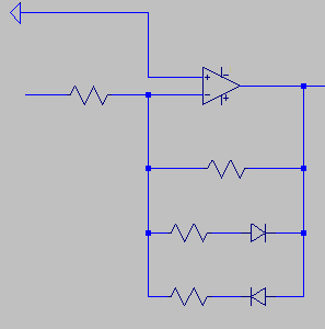
But clipping at the blue line will achieve nothing, what we need to do is clip at some distance BELOW the blue line. So we can modify our peak detector so that it gives us a blue line just underneath the peaks. To do this we’ll make a couple of modifications to our peak detection circuit:

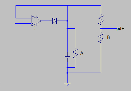
Note in the above circuit we’ve added a resistor in parallel with the capacitor (A). This allows us more fine grain control over how fast the capacitor discharges (more on this below).
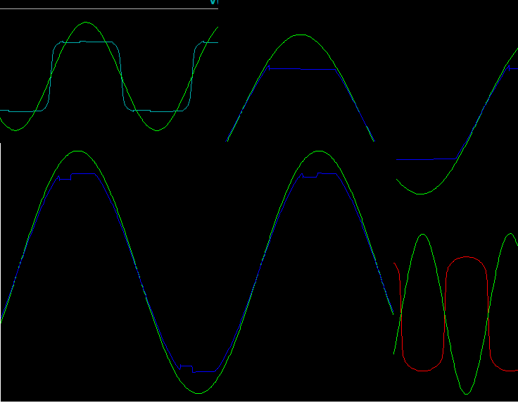
We’ve also added a potential divider (pot) on the output (B). this is what allows us to determine how far below the peaks our blue line will be. The result in something like this:

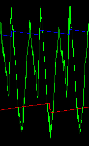
Peak Detection Compromises

Notice in the trace above that the blue line will clip the highest peaks much more than the lower peaks.
Worse yet, the red line (the negative peaks) will completely ignore some of the lower peaks.
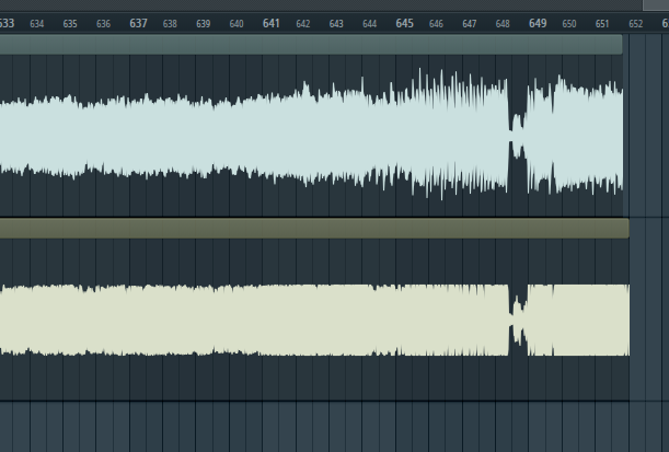
And still worse.. Imagine playing a palm muted ‘chopped’ or staccato phrase on the guitar :

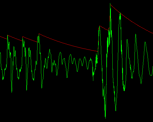
Here we can see that as the guitar signal gets quieter between notes, the peak detection level (the charge in the capacitor) is not falling fast enough to keep up, which means we’ll only be clipping the ‘loud’ parts of the music. We could fix this by reducing the size of the capacitor (or the resistor in parallel with it) but then we might get this opposite situation:

Here we see that reducing the discharge time of the capacitor means that we no longer have a peak detector. Instead we have a simple voltage follower.

Actually clipping the signal

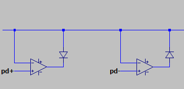
Here we can see how we actually clip the signal. The opamps receive the raw signal and the output of the peak detectors.
Notice that the actual clipping circuit looks exactly the same as a peak detector. That is to say, it’s just a diode in the feedback loop of an amplifier. Perhaps the diode used in the clipper and the peak detector could be combined?

Following a filtered version of the input signal instead

One solution to create a more reliable peak detector may be to not detect the peaks of the original signal which can have a lot of dynamics, but instead detect the peaks of an approximation of the original signal. One idea might be to filter out all of the high frequencies and just follow the general shape of the low frequency signal. To do this we’d create a “low pass filter”. In op-amp world, a low pass filter is just a capacitor in the feedback loop of an op-amp:

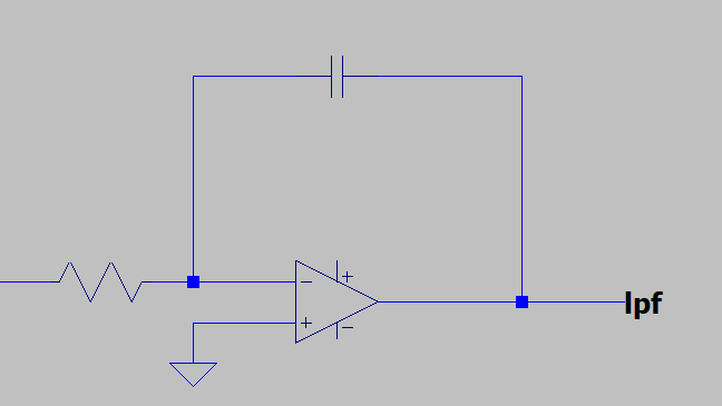
Now if we detect the peaks of the output of the low pass filter and use a smaller capacitor in the peak detector we might have a more responsive and less ‘voltage followy’ clipping line:

Now I’m talking about these situations as if they are problems.
But the real question is, what effect does the discharge rate of the capacitor have on the sound of the fuzz?
Is it better to just chop off the high peaks and leave the lower ones, or is it better to just chop a percentage off each peak? Is it better to chop off a percentage of an averaged (filtered) set of peaks? Or are there still other ways we could approach peak detection and clipping which would produce a more ‘valve like’ sound? Everything I’m talking about here has been done. And you can buy a fuzz, overdrive or distortion pedal that uses the concept. But I want to draw your attention back to the original Big Muff clipping section.

Can you see that what we have is an amplifier that has some diodes and capacitors in its feedback loop? Somewhere in there perhaps might be a low pass filter, clipping diodes, an offset peak detector that sets the clipping level at some pre-determined level?

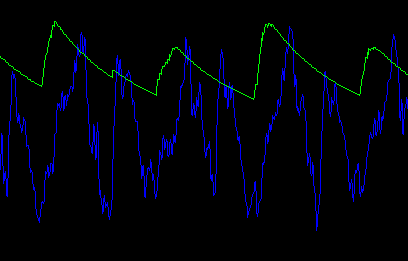
Compression

Moving on.. What if we could make all the peaks the same height by making the loud parts quieter and the quiet parts louder? Clipping a percentage off each peak would then be a trivial task. The act of removing dynamics (the varying amplitudes) from a wave form is called ‘compression’. Here’s an example of a raw signal, and then the compressed version of that signal:

The problem here if we compress our input signal it will loose all it’s dynamic range, which MAY sound bad (it may not also). And in fact if we just went back to only chopping the tops off the biggest waves (having a large capacitor with a slow discharge time) then the effect we’d get would be to chop the large waves to a similar size as the small ones, that is to compress the input signal. Almost all distortion effects based on clipping will naturally ‘compress’ the input signal and we’ve come to actually enjoy this as a bonus side effect.

But what if we wanted to keep the dynamic range. What if we wanted to have quiet bits quiet and loud bits loud, just with some fuzziness? Could we compress the original signal, chop of the tops, and then somehow expanded the signal back out into it’s original dynamic range? This idea is called ‘companding’ (compressing-expanding).
Companding is used in all sorts of effects units particularly old analogue delays. It has the effect of reducing unwanted noise amongst other things.
I’m going to leave this idea of compression before clipping here, except to say you can experiment with it in the LTSpice file below.
I am working on a “companded” overdrive effect and I may write a separate piece on that in the future. There is a fabled schematic design for exactly this dating back some 20 years but I know of nobody who can find the original design, nor has a completed example of the effect.

One last comment on this though. There was a program on TV in the 80’s called ‘Pookisnackenburger – Hell Bent’ in which the immortal line “We don’t want noise reduction, we want noise INDUCTION’ was uttered.
By and large, people don’t want a precise, quiet, meticulously clipped effect. They want something that sounds nasty, like the Big Muff (which is why it’s still selling so well 60 years later). But I’ll continue on.

Doing all this in the modern world of jellybean electronic components, and with perfect hindsight

So what we have in the original Big Muff clipper and pretty much every fuzz, overdrive or distortion that has followed it, is a very clever set of filters peak detectors and clippers squashed down into the minimal set of components. Squashing these components down in this way also adds a lot of weird dynamic features into the mix that we’ve come to like. But it also reduces the amount of variables we have to play with. For example what if we could use a different low pass filter setting for the negative waveform and have some sort of odd asymmetric clipping sound? What if we could vary the envelope filter and therefore the clipping level using an LFO (what would that sound like!?) What if, what if.

So here we have a circuit which expands out all the options into separate op-amp stages which can be tweaked independently to give us maximum control over the end result:

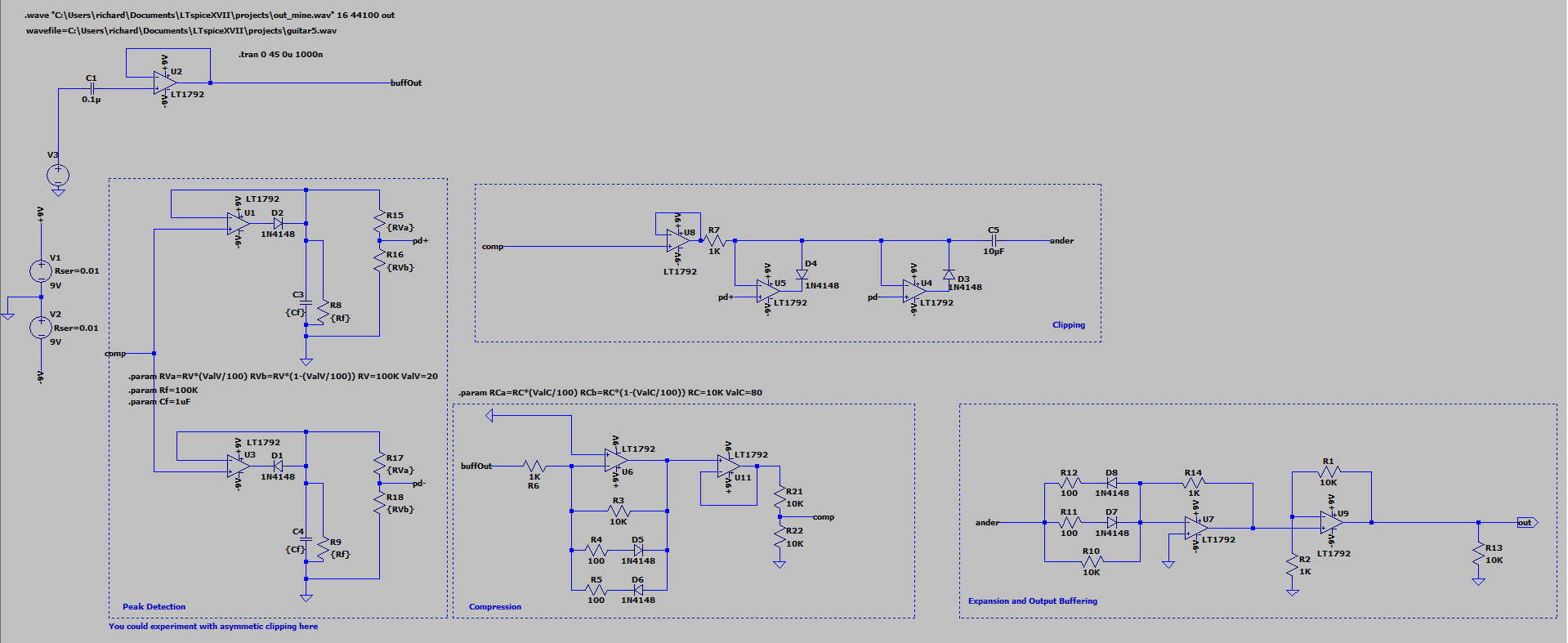
Here is the LTSpice file itself.
You can put your own signal into it and record the output back into a wave (ctrl click on the voltage source V3 to change the input file location)

Here’s what it sounds like (at one example of what it can sound like):
You can if you play with this, get some pretty good results. As I said above, I’m working on an actual pedal which will be based on this approximate design, with a few extra bells and whistles.

Conclusion

Some clever people in the 1960’s managed to create a design for perhaps the most popular guitar effect, and that design has hardly changed since. Why? Well because it works.